Visualizing data can be challenging when it involves more than two dimensions. One of my favourite three-dimensional diagrams is the bubble chart, where the two axes represent two dimensions and the size of the bublles represents the third dimension. But sometimes other types of three-dimensional diagrams squezeed into two dimensions can be helpful.
Recently, I needed to find a way to characterize urban areas in three distinct but related dimensions that can be described by three ratios \(\{\alpha\equiv a/z,\beta\equiv b/z,\gamma\equiv c/z\}\) where \(\max\{a,b,c\}\le z\) and thus the ratios are all between zero and one. Specifically, I was looking to find a diagram that characterizes how dissimilar these regions are. Consider displaying these three ratios in an equilateral triangle with axes A (pointing upward), B (pointing southwest), and C (pointing southeast), as shown below, with side length \(w\) and therefore height \(h\equiv w\cdot\sqrt{3/4}=w\cdot\sin(60^\circ)\). Starting from the center of the equilateral triangle with coordinates \((x_c,y_c)\) and noting that the maximum distance from the centre to each corner is \(l\equiv w/\sqrt{3}\), \[ x = x_c + \frac{w}{2} (\gamma-\beta) \] \[ y = y_c + \frac{w}{\sqrt{3}}\left[\alpha-\frac{1}{2}(\gamma+\beta)\right] \] Another way to describe this is to move \(\alpha\cdot l\) in the direction of A, turn 120° counterclockwise, move \(\beta\cdot l\) in the direction of B, turn another 120° counterclockwise, and move \(\gamma\cdot l\) in the direction of C.
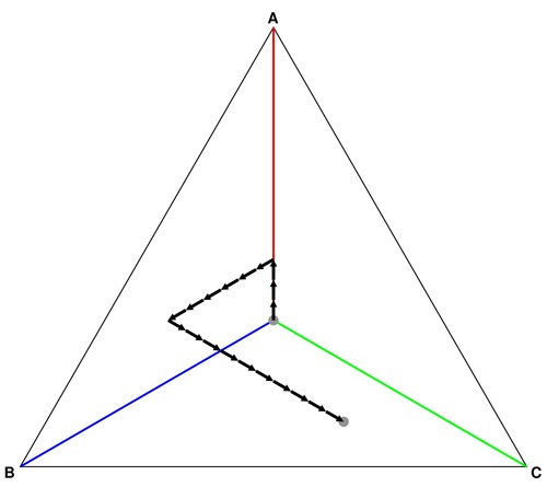
In the example above, there are three arrow movements into direction A, six arrow movements in direction B, and ten arrow movements in direction C. This means that the destination point should be mostly in the (green) area towards C and a little in the direction of (blue) area B.
The distance \(r\) from the center point is given by \[ r=l\cdot\sqrt{\alpha^2+\beta^2+\gamma^2-\alpha\beta-\alpha\gamma-\beta\gamma} \] When dissimilarity is smallest and \(\alpha=\beta=\gamma\), the distance is zero. The more dissimilar the values of the three parameters, the greater the distance. When one of the three measures is equal to one and the other two equal to zero, the distance is largest at length \(l\). It is easily shown that the ratio \(r/l\) is proportional to the standard deviation of the three measures so that \(\sigma\equiv(r/l)\sqrt{2}/3\). These caculations prove that the diagram is indeed a dissimilarity diagram.
Dissimilarity alone could be displayed in a one-dimensional diagram, but the second dimension is crucial as well. It describes the source of the dissimilarity by pointing in the direction of the largest contribution to the dissimilarity.
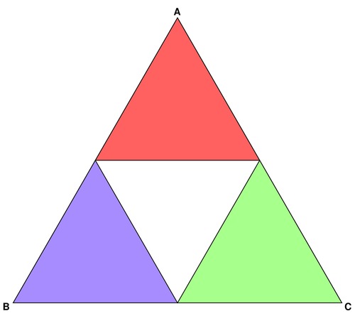
Displaying the target point in the triangular diagram looks a bit dull. It would be nice to give a visual sense of the distance from the center (as a measure of the intensity of dissimilarity) as well as the directionality of the dissimilarity using colours and shades. It makes sense to use primary colours to shade each corner of the equilateral diagram, with white in the middle. Equilateral triangles can be divided neatly into four smaller identical equilateral triangles, as shown in the next step.
It is possible to recursively divide each equilateral triangle into four identical smaller triangles. The next step shows how this works out. One problem to take into account is that the middle triangle points downward instead of upwards.
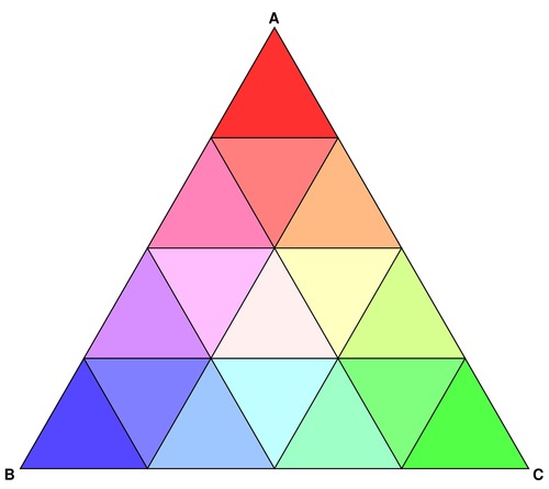
Repeating the recursion twice more and shading each triangle according to its direction and position relative to the centre provides for increasingly smooth shading.
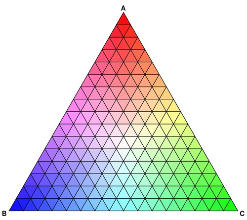
In the last step, the smooth triangular gradient emerges when the recursion level is set to 7. At that point, the triangle is filled with 16,384 small triangles, and that is sufficient to generate the impression of smoothness. For larger triangles or higher resolution, another one or two recursion steps may be necessary.
The last version also displays the points of interest. For example, the V6T district is mostly of type "B", while V5T and V6R are mostly mixtures of types "A" and "C". Region V6H is an A-B mixture, while V6Z is a B-C mixture.

Below is the PostScript code that implements the diagram with a base length of 500 points and outputs the result into an image of 540 by 480 points. There are separate code elements for upward-pointing and downward-pointing triangles. The color shading is based on a formula that calculates the angle and distance from the center using "sethsbcolor". The hue is defined by the angle, which is calculated from coordinates using the "atan" operator. This creates a small problem when both coordinates are zero. I fix that by adding a tiny amount "epsilon" to the y-coordinate, but it can also be fixed with a simple if-then statement checking for both operators being zero. In that case, the hue can be any number because the saturation will be zero (implying white). The saturation level is the relative distance from the centre. If it is more desirable to have more whiteness in the middle, a simple modification is to remove the square root operator in the "fillUp" and "fillDown" functions.
In the PostScript code below I paint all triangles recursively, which means that the larger triangles are painted over by the small triangles. This is a bit inefficient, and you can fix that by activating the "i depth ge { } if" code that I have currently commented out. The advantage of painting smaller over larger triangles is that it removes linear artificats that may appear when the Postscript code is rendered as a raster image.
Recursion is not entirely easy to implement in PostScript, and thus the code involves tail recursion where temporary coordinates are moved onto the stack before the "trifill" routine is invoked for each of the four smaller triangles. Understand the nature of the recursion before you try to modify the code for other purposes.
To adjust the diagram, you need to change the value of the "base" constant, currently 500 points. The diagram is painted with a (20,20) offset.
For putting points in the diagram I use the function "abcz" that has four arguments that define my three ratios \(\{\alpha\equiv a/z,\beta\equiv b/z,\gamma\equiv c/z\}\) along with a label. Rather than calculating the x and y positions exactly, I simply move along the three different directions and rotate 120° each time.
Lastly, you may be curious how I generated the JPEG images based on the above PostScript code. For that I use the ImageMagick software that is widely available freely for many different platforms.