In my recent blog about traffic congestion in Canada I pointed to the dangers of haphazard road tolling for recovering the cost of road improvements (such as a new bridge or tunnel) through a single-point road toll. It sounds simple and straight-forward: make the users of the new infrastructure pay for it. However, it ignores that a toll reshuffles traffic and leads to a suboptimal outcome. Here, I show how this result comes about in a simple microeconomic framework, and I discuss how road tolling can be done better.
Image licensed from iStockphoto.
There is little doubt among economists and traffic experts that road pricing can play an important role in optimizing traffic flows and reducing congestion. However, road pricing can come in many forms and shapes, and it is quite easy to do it wrong and upset many motorists. Road pricing that simply pays for an infrastructure upgrade, such as a bridge or tunnel, seems to be politically appealing because it applies the "user-pays" principle. However, the key economic insight is that any pricing shifts allocation, and people trying to avoid the toll create negative externalities: more congestion elsewhere. Unless the tolled road has no substitutes, single-road tolling is inefficient. Some motorists may say: if I never use the new bridge or tunnel or highway, why should I pay for it? The answer is simple: if you don't pay, your untolled road will get more congested. How much would you be willing to pay to stay on a less congested road? You will get something in return for what you pay.
This blog involves some math. If you are simply interested in the policy discussion, jump straight to the last section below.
A simple two-road traffic congestion model
Let us consider a simple model with two parallel roads, 1 and 2, of equal length. They are substitutes for each other reaching the destination, although they may be subect to different speed limits and capacity constraints. Driving on these roads connects the same origin and destination over a distance \(D\), and drivers can choose to drive on either one. Road \(i\) has a nominal speed (the speed limit or effective speed without congestion) of \(v_i\) km/h and a capacity of \(c_i\) vehicles. The time \(t_i\) it takes to reach the destination is a function of the speed and congestion: \[ t_i=\frac{D}{ v_i(1-n_i/c_i)^{\xi}} \] This functional form is a reasonable approximation and captures the essence of congestion: more traffic, slower speed. (It is a simple one-parameter function; more realistic versions would include multiple parameters.) Road \(i\) is occupied by \(n_i\le c_i\) vehicles, and let \(n\equiv n_1+n_2\) be the total number of vehicles on the go. Furthermore, \(0<\xi<1\) is a parameter that determines the road's congestivity. The larger the parameter, the longer it takes to get to the destination for the same level of congestion. The ratio \(u_i=n_i/c_i\) is also the capacity utilization rate. The image below shows what the road congestion function looks like for a road with maximum speed of 60 km/h for different values of \(\xi\). When the road reaches its capacity limit and cars are lined up bumper to bumper, speed drops to zero.
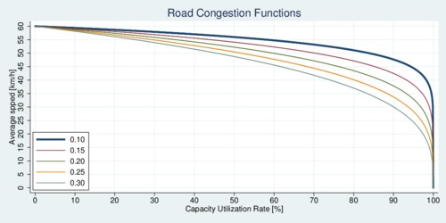
click on image for high-resolution PDF version
Motorists value their time at a rate \(w\) in dollars per hour. Let us asume that all motorists are the same, to keep our analysis simple. Then the total cost of time spent in traffic is \(\Omega=w(n_1 t_1+n_2 t_2)\). We want to minimize this cost by distributing our motor vehicles \(n_i\) in an optimal fashion. If individual motorists make this choice rather than a central planner, motorists choose whichever road is faster. This imposes a no-arbitrage condition that equalizes the time on each road so that \(t_1=t_2\). We can solve this no-arbitrage condition for the proportion \(\alpha\equiv n_1/n\) of vehicles on road 1. Let \(\beta\equiv c_1/c\) be the simple capacity share of road 1 with \(c\equiv c_1+c_2\), and furthermore denote with \[ \zeta\equiv\frac{ c_1v_1^{-1/\xi}}{c_1v_1^{-1/\xi}+c_2v_2^{-1/\xi}} =\frac{c_1}{c_1+c_2 (v_1/v_2)^{1/\xi}} \] the speed-adjusted capacity share of road 1. Note that \(\zeta=\beta\) when both roads have the same nominal speed. If road 1 is faster than road 2, then the term \((v_1/v_2)^{1/\xi}\) makes the capacity of road 2 appear smaller in speed-adjusted terms. For example, the expression \((70/50)^{1/3}=0.364\) suggests that a road with a speed of 50 km/h has a speed-adjusted capacity of only 36.4% of a road with 70 km/h. (Even though road 1 is only 40% faster than road 2, road 2 will experience more rapid congestion for the same amount of traffic.)
Applying these definitions to the no-arbitrage condition that defines motorists' choices, it turns out that \[\alpha=\beta + (\beta-\zeta)\left(\frac{c-n}{n}\right)\] At first, motorists only take the faster and bigger roaad, which we assume to be road 1 with \(v_1>v_2\) and \(c_1>c_2\). This continues until road 1 reaches a capacity utilization of \(u_1=1-(v_2/v_1)^{1/\xi}\). As more traffic uses road 1, \(\alpha\) decreases from 100% down to \(\beta\). With our assumptions about roads 1 and 2, it can be shown that \(\beta>\zeta\). The expression \((c-n)/n>1\) is the ratio of unused capacity \(c-n\) to used capacity \(n\).
Consider a numerical example with two roads of 12km, an hourly capacity of 15,000 and 5,000 vehicles, nominal speeds of 70 and 50 km/h, a total flow of 16,000 vehicles per hour, and a congestivity parameter of \(\xi=1/3\). The capacity share \(\beta\) of road 1 is thus 75%. However, taking congestion into account (and noting that \(\zeta=0.522\), motorists will choose the faster road 1 more, and thus \(\alpha=\)80.7%. Road 1 has a utilization rate of 86%, while road 2 has a utilization rate of only 62%. Motorists' individual choices are not necessarily optimal. An urban planner would have shifted motorists a little; the optimal \(\alpha\) that minimizes \(\Omega\) is 76.7%. However, the central planner does not have a policy tool to balance traffic. The diagram below illustrates the welfare losses as roads approach the capacity limit. The horizontal axis shows the share \(\alpha\) of traffic on road 1, while the vertical axis shows the welfare loss relative to the optimum in percent.
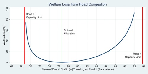
click on image for high-resolution PDF version
You probably wonder why motorists' road choice that equalizes travelling time is not optimal. At the margin, shifting some drivers from the slightly overcongested road 1 to the less congested road 2 speeds up traffic more for the many drivers on road 1 than it reduces spped for the fewer drivers on road 2. However, motorists would not volunteer to be the ones assigned to the slower road. So without a mechanism to induce motorists into the optimal choice, the emerging traffic pattern is slightly sub-optimal.
A tolled and an untolled road
Now the government decides to spend \(F\) to improve road 1; perhaps this is a new bridge, or tunnel, or interchange. To recover the cost of this improvemnt, the government charges a road toll \(\tau_1=F/n_1\), but only on road 1 and thus only the \(n_1\) motorists who use that road pay. Motorists again equalize the cost of driving on either road so that \( w\cdot t_1+\tau_1 =w\cdot t_2 \). This no-arbitrage conditions means that motorists will continue taking the cheaper route until both road are equally costly. The notion of "cheaper" entails both the time cost, priced at \(w\), and the toll \(\tau_1\). The obvious outcome of the single-road toll is that congestion decreases on road 1 but congestion increases on road 2. Let's say the toll is $4 per trip, and the wage rate is $20. This means that the typical motorist is indifferent between paying the toll and sitting 12 more minutes in traffic. The outcome on traffic flows can be quite significant.
Consider again the numerical example. Assume that the hourly cost to cover is $30,000 (about $267mio annually). Solving the new no-arbitrage condition reveals that 74.7% of motorists now take the tolled road 1, down from 80.7%. That is, 6% of motorists have shifted to the alternative untolled road. Both roads now have a capacity utilization of about 80-81%. The road toll turns out to be $2.51 per trip on road 1, which is equivalent to spending 7.5 minutes longer on the road. The total value of time lost in traffic comes to $103,473 per hour. The toll has had a beneficial effect by reducing the traffic on congested road 1 a bit, and in the numerical example, that makes the drivers better off overall (the welfare loss drops from 3.2% to 0.9% relative to the optimum). Going from no road tolling to some road tolling can indeed be beneficial. But can tolling both roads lead to a better outcome yet?
Both roads tolled
Now assume that the government tolls both roads to recover its costs for upgrading road 1, but at different rates \(\tau_1\) and \(\tau_2\). The urban planner uses this policy tool to direct traffic to minimize \(\Omega\) with respect to the two road tolls \(\tau_1\) and \(\tau_2\), subject to the no-arbitrage condition that equates the cost of both roads for each driver \(w\cdot t_1 + \tau_1 = w\cdot t_2 +\tau_2\), and subject to the cost-recovery constraint \(n_1\cdot\tau_1+n_2\cdot\tau_2=F\) for building the road upgrade. The two constraints imply that the difference in tolls is equal to the value of the time difference \(w(t_1-t_2)=\tau_2-\tau_1\) and therefore each toll is given by: \[ \tau_1=F/n-(1-\alpha)(t_1-t_2)w \] \[ \tau_2=F/n+\alpha(t_1-t_2)w \] The urban planner needs to figure out the optimal \(\alpha\), which is determined by the first-order condition for minimizing \(\Omega\). This is a non-linear equation, unfortunately, and can only be solved numerically. It turns out that the optimal tolls are $2.24 and $0.69 for roads 1 and 2 respectively, which leads to an optimal distribution of \(\alpha=\)76.6%, which is the optimum (see chart above). The total value of time lost in traffic is now $102,504 per hour, abut 1% less than when only one road is tolled.
The gain from tolling both roads appears minute in the above numerical example. The example was chosen conservatively. Now change a few of the paramters. Assume both roads have the same effective speed of 70 km/h, and leave capacity unchanged. The optimal division of traffic is now \(\alpha=\)75% for the bigger road 1, with a total cost of time in traffic of $93,804. With a single toll of \(\tau_1=\)$2.64, this cost rises to $100,261, a 7% welfare loss compared to the optimum as about 4% of vehicles shifting to the non-tolled road \((\alpha=0.711)\). With an equal toll of $1.875, however, the optimal allocation of traffic is restored. Clearly, the single toll makes things worse for motorists than optimal tolls on both roads.
The two equations above that define the optimal tolls are generic. They also work when \(F=0\). In that case, one road would be tolled, while the other would actually pay drivers to use it. This revenue-neutral method would shift traffic in such a way that it makes drivers pay for getting to work faster and compensate driveres for getting to work slower. This is a general principle of efficient road tolling.
Which of the two roads is tolled more than the other does not depend at all on where the road improvement was provided. The road toll recovers the funds needed to pay for the improvement, but the distribution of the toll depends entirely on optimizing traffic flows, which is determined by the time difference \(t_1(\alpha)-t_2(\alpha)\) with \(\alpha\) chosen to minimize \(\Omega\).
Policy conclusions: what are the key insights?
‘Smart road pricing takes into account all traffic flows; user-pays pricing that doesn't is haphazard.’
The model and numerical examples make it clear that road tolling can be used well or used badly. The erroneous method uses road tolling to recover investment costs in a simple "user pays" approach. Tolling a single road diverts traffic as motorists adjust to balance their time-plus-toll cost across different road choices. It is also not optimal to toll all roads equally. If tolls are used, they need to take into account the congestion on all roads. Individual tolls need to be set so that road utilization is optimized and time wasted in traffic is minimized. Smart road pricing takes into account all traffic flows; user-pays pricing that doesn't is haphazard.
‘Road pricing should be broad but with low individual tolls.’
Simple road tolling only makes sense when there are no alternatives, or the alternatives entail lengthy detours. When British Columbial tolled the 186-km Coquihalla highway between Hope and Kamloops between 1986 and 2008, cars were tolled $10 per trip. After the highway was fully paid for, the province discontinued the toll. The province of British Columbia has announced that the George Massey Tunnel will be replaced with a bridge, and that this bridge will be tolled like the Port Mann bridge. While tolling can make eminent sense, it needs to be done right by taking all traffic flows into account. This means that other bridges and highways should have appropriate tolls as well in order to minimize travel time overall. If the province relies increasingly on road pricing—and there are good arguments in favour of this approach—it needs to be done right. Road pricing should be broad, helping to fine-tune traffic flows, with low individual tolls.
The model used above was simplified in some important ways. For example, it assumes that trip demand is perfectly inelastic. Road pricing also lowers demand for road trips. The model also ignores the heterogeneity of motorists. Some people are in a hurry and are willing to pay more, and others are less in a rush. Road pricing needs to take this heterogeneity into account, and this also has different distributional outcomes. This will be the topic of a forthcoming blog. Also, congestion peaks during rush hour. Should tolls vary minute-by-minute? The merits of dynamic tolling, as well as the practical difficulties with that approach, are further topics for my blog. Stay tuned for more.