My last blog on Haphazard road tolling introduced a simple model of road congestion and showed that optimal road tolling is aimed at reducing traffic congestion rather than recovering the cost of road upgrades such as bridges or tunnels. Today's blog looks at another question about road pricing: how does road pricing interact with public transit?
Image: Translink
Consider a simple economic model of public transit and a congested road that both cover a distance \(D\) and operate at speeds \(v_0\) for transit and an uncongested speed \(v_1>v_0\) for the road. The road has a capacity of \(c_1\), and public transit has a larger capacity \(c_0>c_1\). Travel time on public transit is \(t_0=D/v_0\), while travel time on the road is given by the simple single-parameter congestion function \[ t_1=\frac{D}{ v_1(1-n_1/c_1)^{\xi}} \] where \(n_1\) is the number of vehicles on the road and parameter \(0<\xi<1)\) identifies the congestivity of the road. There are \(n_0\) passengers taking public transit so that \(n=n_0+n_1\) is the total number of trips taken, and \(\alpha\equiv n_1/n\) is the share of road users. The urban planner's objective is to minimize total travel time \[\Omega = n_0 t_0 + n_1 t_1 \] It turns out that optimizing this function means putting a fixed number of users on the road regardless of the total number of travelers. Assuming that public transit can carry a growing number of passengers (running longer trains or more often), welfare loss is minimized when the road carries an optimal number of passengers. The diagram below illustrates the welfare loss relative to the optimum for different rates of utilization of the road [\(n_1/c_1\) in percent]. At first, shifting more users onto the road improves welfare as the uncongested road is faster. Eventually, more congestion slows down traffic and welfare decreases. The green vertical line shows the optimum (at 52.4%), and the red line shows the utilization (81.3%) when commuters access the road freely (81.3%) and equalize travel time on both transportation modes. The key insight here is that travel time equalization is suboptimal. It is optimal to shift more road users to public transit. Although individually that makes these commuters worse off because they take longer to reach work, the welfare gain from faster road traffic by the remaining road users is larger than the welfare loss from the commuters who are shifted to public transit. Of course, who wants to volunteer traveling slower? The economic magic that makes that happen is to make both trips equally costly: compensate the people who use public transit for the longer trip time with a lower cost. When commuters choose the travel mode, they don't choose the faster mode but the cheaper mode until cost equalizes across modes.
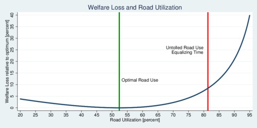
click on image for high-resolution PDF version
The numbers used in this numerical example are road length \(L\)=12 km, transit speed \(v_0\)=40 km/h, uncongested road speed \(v_1\)=60 km/h, road capacity \(c_1\)=3000 vehicles, congestivity parameter \(\xi\)=1/3, cost of time \(w\)=25 $/hr, fuel cost \(f\)=$5/hr, and transit cost \(r\)=$3/hr.
As a tool to influence traffic flow, the urban planner can decide to levy a toll \(\tau\) on each road user. To make this toll revenue-neutral to the government, the toll collected is paid out as a per-trip subsidy \(\rho\) to each user of public transit so that \(n_1\tau=n_0\rho\). Each of the \(n\) commuters now has to decide on the transportation mode, and this will equalize transportation costs for each mode \[ w\cdot t_0 + r - \rho = (w+f)\cdot t_1 + \tau \] where \(w\) is the cost of time in $/hour, \(r\) is the cost of each train trip, and \(f\) is the fuel cost (also in $/hour, rather than $/km).
The revenue-neutral tolling condition implies \(\rho=\tau\cdot\alpha/(1-\alpha)\), and inserting this into the no-arbitrage condition for transportation mode choice provides a solution for the optimal toll \(\tau^\ast(n)\) as a function of the total traffic volume \(n\): \[\tau^\ast(n)=(1-n_1^\ast/n)[w\cdot t_0 +r-(w+f)\cdot t_1(n^\ast_1)] \] There is a useful insight in this solution: the optimal toll increases with overall traffic volume. With road capacity fixed, an increase in the number of commuters will increase the road toll to ensure that all the extra commuters don't increase road use but are all shifted to public transit. The diagram below shows the optimal road toll and optimal transit subsidy as a function of the traffic volume as a percentage of the road capacity.
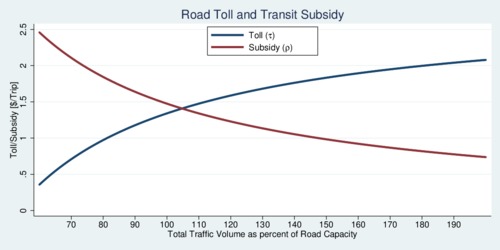
click on image for high-resolution PDF version
To summarize, the key insight is that road tolling should be linked to subsidizing public transit. Rather than using road pricing simply to pay for road infrastructure, road pricing can help move traffic from roads to public transit in order to maximize social welfare and reduce the time people waste in congested traffic. The ideal instrument is revenue-neutral: road users enjoy faster commutes, but pay transit users for their slightly slower commute.
It is important to keep in mind that road pricing will affect different people in different ways. Some road users don't have the choice to take alternative modes of transportation. They are stuck with driving their car and paying the road toll. The road price is unable to change their transportation mode choice. For these commuters, a road toll remains a tax. This is a problem that requires fixing. In the long term, road pricing generates an incentive to move closer to work, but this may not be cheaper if housing is expensive closer to the urban core. In the short term, the task is to price-differentiate between commuters who could use transit and those who clearly cannot. This requires another instrument, such as a rebate for long-distance commuters. In effect, this is already something that is done in Metro Vancouver, albeit crudely. Gasoline taxes are lower outside Metro Vancouver. Long-distance commuters get some compensation through this channel, although not fine-tuned based on their commuting trip. You can probably guess where the direction is going for truly smart road pricing: a different price for each trip depending on origin and destination, and time of travel. Can it ever be done? Technically, with GPS data it is possible to solve this problem. However, that type of precise trip data would quickly become a major invasion-of-privacy issue. If perfect road pricing is not possible, it is still possible to come up with good approximations, especially as commuters travel through multiple traffic choke points. Smart road pricing, thus, is the best road pricing we can do without invading privacy unduly while improving traffic flows and sharing financial burdens fairly. More on this in my forthcoming blogs.