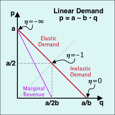
The topic of today's blog is esoteric: how economists model consumer demand when we teach about it in our microeconomics courses. I have just been teaching a course on managerial economics, and I was reminded how much we stick to traditional forms of modeling demand. Economists like to work with linear demand because (a) it is graphically simply to reproduce, and (b) it usually leads to simple analytic solutions for understanding markets. For practical purposes, we follow the tradition of using an inverse demand function of the form \[p=a-b\cdot q\] where \(p\) is price in $/unit, \(q\) is quantity in units, \(a\) is the maximum price when demand is zero, and \(b\) is the slope of the inverse demand line. This looks like what you see in the diagram on the right above, which is a familiar sight to all economics students. The (negative) price elasticity of demand is given by \[\eta\equiv \frac{\partial q}{\partial p}\frac{p}{q}=-\frac{p}{a-p}\] Demand is inelastic below a price of \(a/2\), and it is elastic above \(a/2\). The price elasticity is equal to one at \(a/2\). Furthermore, consumer surplus at a given quantity \(q^\ast\) is neatly \[\mathrm{CS}=b\cdot(q^\ast)^2\] A monopolist only operates on the elastic part of the demand curve as marginal revenue is positive only when quantity is smaller than \(a/2b\). The popularity of linear demand is easy to see in the diagram: it is easy to draw, and marginal revenue is simply doubling the slope of the demand curve. However, one of the problems with linear demand arises when we want to compare two markets. What captures the size of markets when we have two markets with parameters\(\{a_1,b_1\}\) and \(\{a_2,b_2\}\), respectively? We want something expressed in "units", so one possibility is \(a_1/b_1\) and \(a_2/b_2\), which captures the market saturation points (when price is zero). With the traditional preference of using inverse demand functions, this requires two parameters and thus becomes a little less intuitive.

The other popular demand function is the simple log-linear demand function \[\ln(q)=\ln(a)-b\cdot\ln(p) \quad\Leftrightarrow\quad q=\frac{a}{p^b}\] that has iso-elastic demand \(\eta= -b\). Unfortunately, consumer surplus is hard to work with here. It is infinite when demand is price inelastic, and when demand is price elastic (i.e., when \(b>1\)) it is given by \[\mathrm{CS}= \frac{q^\ast}{b-1}\left(\frac{a}{q^\ast}\right)^{1/b}\] which is clearly a bit unwieldy.

Negative exponential demand is an often overlooked alternative. However, it has a number of attractive properties that make it very useful in many circumstances. It is primarily written not as an inverse demand function, but directly as a demand function: \[q=a\cdot\exp(-p/b)\] Thus, inverse demand is \(p=b\cdot\ln(a/q)\). Here the parameters \(a\) and \(b\) take on a different meaning. Parameter \(a\) is a type of market size (with physical dimension "units"); it is the market saturation quantity when the good is free. Parameter \(b\) is measured in $/unit and turns out to be the price at which demand becomes elastic; it is the "unit elasticity price". The price elasticity of demand is simply \[\eta = -p/b\] The price elasticity again starts at zero when the price is zero and becomes more elastic, but proportional to price. When \(p=b\), the elasticity is exactly equal to unity (–1). The higher the price, the more elastic the demand. Marginal revenue is also easy to express: it is simply \(\mathrm{MR}=p-b\), which means that it is the demand curve shifted down by \(b\). The diagram below illustrates an example with parameters \(a\)=100 units and \(b\)=$5/unit. In the diagram, the purple curve describes marginal revenue. It reaches zero at a quantity \(a/e\), where \(e\) is Euler's constant (2.718). In comparison to linear demand, where MR is zero at half the saturation quantity, MR is zero for negative exponential demand at 36.788% of saturation demand. Neatly, the gap between the demand curve and the MR curve is always the same amount \(b\).

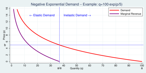
click on image for high-resolution PDF version

A simple trick turns the demand and MR curve back into a more familiar linear shape. Simply scale the horizontal axis logarithmically as shown in the next diagram. Then the demand and MR curves turn back into straight lines, with the MR curve offset from the demand curve by a fixed width equal to \(b\). The two lines are perfectly parallel.

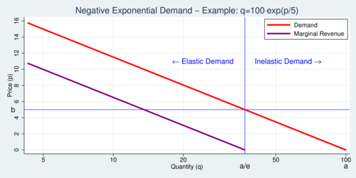
click on image for high-resolution PDF version

Consumer surplus is also a very convenient expression. \[\mathrm{CS}=\int_0^{q^\ast} b\,\ln(a/q)\,\mathrm{d}q=b\cdot q^\ast\] It is directly proportional to the equilibrium output \(q^\ast\). When analyzing a welfare effect where output depends via price on a tax variable \(\tau\), then the welfare elasticity \[\frac{\partial\mathrm{CS}}{\partial\tau}\frac{\tau}{\mathrm{CS}}= -\frac{p}{b}\left[\frac{\partial\mathrm{p}}{\partial\tau}\frac{\tau}{p}\right] =\eta\cdot\theta\] where \(\eta\) is the (negative) price elasticity of demand and \(\theta\) is the (positive) tax-elasticity of price (i.e., the pass-through).

Negative exponential demand also generates relatively easy expressions for a monopoly where marginal cost (MC) is fixed at \(c\). It turns out that the optimal solution implies a price \[p^\ast=b+c\] with quantity \[\frac{q^\ast}{a/e}=\exp\left(-\frac{c}{b}\right)\in(0,1]\] The ratio on the left hand side has a useful interpretation. It is the share of optimal output with respect to the maximum feasible output \(a/e\), as the latter is determined by the requirement that marginal revenue is positive. The expression on the right hand side is also intuitive to interpret. The ratio \(c/b\) is the ratio of marginal cost relative to the unit-elasticity price.

Returning to the issue of comparing markets, the negative exponential demand setup identifies market size through the single parameter \(a\). Unlike linear demand, it does not depend on intercept and slope. It is intuitive to compare markets of different size \(a_i\) while still assuming that consumers behave similarly in a proportionate way and have identical \(b\). As the equation above for the monopoly solution illustrates, a change in \(a\) simply scales up output in proportion when \(b\) and \(c\) are fixed.

In the conventional linear demand specification where monopoly output is \(q^\ast=a/2b-c/2b\), the metric \(a/2b\) captures market size similar to \(a/e\) in the negative exponential case. This is of course merely a result of our convention to write inverse linear demand in this particular form. If we had written linear demand as \(q=a-p/b\) and inverse demand as \(p=b\cdot(a-q)\), then \(a\) is also an intuitive market size measure. In our diagrams we would need to relabel the intercept as \(a\cdot b\), while the slope would remain \(-b\). It would be more intuitive that way, I think. We could go one step further and write linear demand as \(q=a(1-p/2b)\) or \(p=2b(1-q/a)\). This is the form closest in spirit to the negative exponential demand function and the related interpretation of coefficients. Here, \(a\) is also saturation demand, and \(b\) is again the unit-elasticity price expressed in $/units. In our linear-demand diagrams, the intercept becomes \(b\) and the slope becomes \(-2b/a\). The price elasticity of demand is then \(\eta=-p/(2b-p)\), which is equal to –1 when \(p=b\). The key idea is to give meaning to the parameters \(a\) and \(b\) rather then treating them simply as "intercept" and "slope" of the demand curve. If a class of markets has the property that demand is inelastic at low prices and becomes more elastic at high prices, then the concept of a "unit elasticity price" as a reference price makes intuitive sense. The downside of this way of writing linear demand is that algebraic expressions for a monopolist's profit maximum get a bit more complicated. This brings me back to looking at the algebraic virtues of negative exponential demand.

Negative exponential demand is also quite useful in the context of an oligopolistic Cournot model where \(n\) producers have costs \(\{c_1,c_2,\ldots,c_n\}\) with average cost \(\bar{c}= \sum_i c_i/n\) and total output \(q=\sum_i q_i\). Then maximizing profits yields total output and prices: \[q=\frac{a}{\exp\left(1/n+\bar{c}/b\right)} \quad\mathrm{and}\quad p=\bar{c}+\frac{b}{n}\] These expressions are not particularly difficult in comparison to the solution for linear demand models. I find the price outcome is easier to interpret than in the linear case: price is average cost plus a mark-up that diminishes inverse-proportionally with the number of firms. The equilibrium market share of each firm is \[\frac{q_i}{q}=\frac{1}{n}+\frac{\bar{c}-c_i}{b}\] This solution is independent of the overall market size \(a\) and instead depends simply on the cost structure and the unit-elasticity benchmark price \(b\).

To summarize, negative exponential demand is not much more challenging mathematically than linear demand, and in fact it has some nice features. It has a particularly simple and intuitive welfare measure (proportional to output), and it has a simple and intuitive elasticity function (proportional to price). Its marginal revenue function is simply a fixed distance to the demand function, and the two parameters have intuitive interpretations as saturation output and as unit-elasticity price. Perhaps negative exponential demand should receive more attention than it usually does.

And maybe, just maybe, the reason why economists like linear demand so much is that we're better at drawing straight lines instead of gently-sloping curves.

Empirically, linear demand is neither more nor less useful than negative exponential demand. We usually observe only small variations in price and quantity, and thus either demand form provides a reasonable numerical approximation.