Linear demand has had a long history in economics because it is particularly simple to work with analytically and visually. In its normalized form, linear demand can be written as \[\frac{p}{p^\circ}+\frac{q}{q^\circ}=1\] where price \(p\) and demand \(q\) are related to each other through the zero-price limiting demand \(q^\circ\) and the zero-quantity limiting price \(p^\circ\). Analytic tractability comes from the linearity combined with the need to have only two parameters, \(q^\circ\) and \(p^\circ\). The above form gives rise to the conventional inverse demand function \(p=p^\circ-(p^\circ/q^\circ)q\) with intercept \(p^\circ\) and slope \(p^\circ/q^\circ\).
Linear demand can be generalized by introducing a dimensionless curvature parameter \(\theta\) that leads to a more flexible demand system \[\frac{p}{p^\circ}+\left(\frac{q}{q^\circ}\right)^\theta=1\] that nests linear demand with the special case \(\theta\!=\!1\). Of course, generalized linear demand is no longer linear except in this special case. Generalized linear demand allows both for concave demand \((\theta\!>\!1)\) and convex demand \((\theta\!<\!1)\). I have not found a discussion of this demand system in the literature, and thus assume that the discussion here is indeed novel. Essentially, moving from a two-parameter to a three-parameter demand system opens up significantly more flexibility for identifying important relationships.
Today's blog connects to my discussion about the virtues of negative exponential demand in 2018. There I pointed out some of the analytic and expositional advantages of using a specific alternative functional form instead of linear demand. Generalized linear demand lacks some of the analytic simplicity of negative exponential demand, but due to its use of three parameters provides significantly more potential for fitting to the data meaningfully. The analytics, as shown below, are not unwieldy.
Introducing arbitrary curvature into a demand system has important policy implications. If we use demand systems for welfare analysis where we quantify consumer surplus, producer surplus, and deadweight losses, then omitting curvature can lead to serious underestimation or overestimation of policy effects.
This generalized linear demand system has \[\begin{eqnarray} p&=& p^\circ\left[1-(q/q^\circ)^\theta\right]\\ q&=& q^\circ\left(1-p/p^\circ\right)^{1/\theta} \end{eqnarray}\] as the inverse and direct demand functions, respectively. The price elasticity of demand is thus given by \[\eta\equiv\frac{\mathrm{d}q}{\mathrm{d}p}\frac{p}{q} =-\frac{p}{p^\circ-p}\left(\frac{1}{\theta}\right)<0\] The elasticity reaches negative unity at \[\begin{eqnarray} p^\triangle\equiv \left.p\right|_{\eta=-1} &=& p^\circ\,\theta/(1+\theta) \\ q^\triangle\equiv \left.q\right|_{\eta=-1} &=& q^\circ\,(1+\theta)^{-1/\theta} \\ \end{eqnarray}\] which in the case of linear demand (\(\theta\!=\!1\)) implies the familiar \(\{q^\circ/2,p^\circ/2\}\) location. When the price is higher than \(p^\triangle\), demand is elastic, and when it is lower, it is inelastic.
The diagram below illustrates a concave example of a generalized linear demand function with curvature parameter \(\theta=3\). The horizontal and vertical thin lines indicate the unit-elasticity levels \(p^\triangle\) and \(q^\triangle\). The corresponding marginal revenue curve is shown in purple below the blue demand curve. The horizontal and vertical lines show the location of unit elasticity on the demand curve.
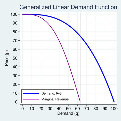
click on image for high-resolution PDF version
The next diagram illustrates a variety of generalized linear demand functions for curvature parameters from 0.5 to 5.0, showing that the functional form can easily generate convex and concave versions.
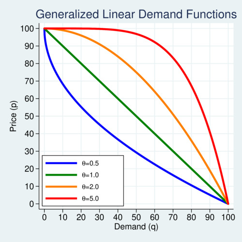
click on image for high-resolution PDF version
Under perfect competition, price equals marginal cost (\(p^\ast_C=c\)) and therefore \[q^\ast_C=q^\circ\,\left(1-\frac{c}{p^\circ}\right)^{1/\theta}\] The corresponding consumer surplus is \[\mathrm{CS}_C= p^\circ q^\circ\frac{\theta}{1+\theta}\left(1-\frac{c}{p^\circ}\right)^{1+1/\theta}\]
It can be shown that \(\partial\mathrm{CS}_C/\partial\theta>0\), which has important implications for policy analysis. If \(\theta>1\) and demand is concave, consumer surplus is larger than when demand is linear. Conversely, when \(\theta<1\) and demand is convex, consumer surplus is smaller than when demand is linear.
Under monopolistic competition, the marginal revenue function becomes \[\mathrm{MR}=p^\circ\left[1-(1+\theta)\left(\frac{q}{q^\circ}\right)^\theta\right]\] which in the linear demand case leads to the familiar \(\mathrm{MR}=p^\circ(1-2q/q^\circ)\) where the slope of marginal revenue is double the slope of the inverse demand curve. The monopolistic profit maximization problem \(\pi=[p(q)-c]q\) has the equilibrium solution \[\begin{eqnarray} q^\ast_M &=& q^\circ\,\left(\frac{p^\circ-c}{p^\circ(1+\theta)} \right)^{1/\theta} \\ p^\ast_M &=& \frac{c+\theta p^\circ}{1+\theta}\\ \eta^\ast_M&=&-\frac{c+\theta p^\circ}{\theta(p^\circ-c)} \end{eqnarray}\]
The producer surplus (profit) is thus given by \[\mathrm{PS}_m=p^\circ q^\circ\theta\left(\frac{1-c/p^\circ}{1+\theta}\right)^{1+1/\theta}\] while the consumer surplus is given by \[\mathrm{CS}_m=p^\circ q^\circ\frac{\theta}{1+\theta}\left(\frac{1-c/p^\circ}{1+\theta}\right)^{1+1/\theta}\] which also implies that the ratio of consumer surplus to producer surplus is \[\frac{\mathrm{CS}_m}{\mathrm{PS}_m}=\frac{1}{1+\theta}<1\] Under linear demand, the monopolistic producer surplus is twice as large as the consumer surplus, but as \(\theta\) increases and demand becomes more concave, the relationship improves in favour of the producer.
The deadweight loss (DWL) is the inefficiency area \(\mathrm{CS}_c-(\mathrm{CS}_m+\mathrm{PS}_m)\) and is given by \[\mathrm{DWL}_m= p^\circ q^\circ\frac{\theta}{1+\theta}\left(1-\frac{c}{p^\circ}\right)^{1+1/\theta}\left[1-\frac{2+\theta}{(1+\theta)^{1+1/\theta}}\right]\] which in the case of linear demand is the familiar expression for the size of the Harberger triangle: \[\left.\mathrm{DWL}_m\right|_{\theta=1}=\frac{p^\circ q^\circ}{2}\left(\frac{1-c/p^\circ}{2}\right)^2\]
It is interesting to investigate how much the demand curvature affects the size of the DWL relative to the linear case, so \(100\%\cdot[\mathrm{DWL}_m(\theta)/\mathrm{DWL}_m(1)-1]\). The last figure below shows the magnitude of mismeasurement of DWL that can be attributed to demand curvature.
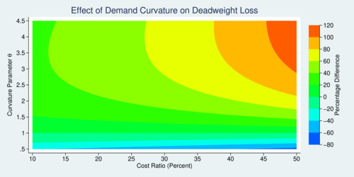
click on image for high-resolution PDF version
If the cost ratio \(c/p^\circ\) is small, the distortions to DWL are small. The distortions can get fairly large (over 100%) if the curvature is highly concave (\(\theta\) over 3) or the cost is higher than about 45% relative to the price \(p^\circ\) where demand drops to zero.
The purpose of this exercise was to show that deviations from linear demand can have large effects on welfare analysis and related policy areas, such as competition policy. Demand estimation should therefore carefully assess the demand curvature rather than imposing linearity for convenience.