Production methods in the 21st century are characterized increasingly by situations where marginal costs are effectively zero and the entire production cost is effectively a fixed cost. Examples abound in the world of digital media, but they can also be found in the energy industry. Generation of electricity from wind, sun, hydro, or geothermal energy falls into that category. The production cost is virtually all fixed cost of building the generator, and once in operation, the cost of production is zero. After all, sun, wind, hydro, and geothermal energy are free. The phenomenon is important enough to have made it into a book: Jeremy Rifkin's The Zero Marginal Cost Society.

Zero marginal cost production plays tricks with what we know from conventional market situations. Profit maximization tells us that marginal revenue (MR) should equal marginal cost (MC), but when marginal costs are zero, we produce where marginal revenue is zero. But in that case a business could easily make losses if it fails to cover its fixed cost, or the business may not enter in the first place.

Consider a simple model where price \(p\) is a linear function of quantity \(q\) so that \(p=a-b\cdot q\). When marginal costs are zero, marginal revenue is zero as well, and thus a firm produces quantity \(q^\ast=a/(2b)\) and charges price \(p^\ast\equiv p(q^\ast)=a/2\). But this price must be large enough to cover average cost: \(p^\ast\gt f/q^\ast\), where \(f\) is the fixed cost of production. Therefore, fixed costs must be sufficiently small: \(f\lt (a/2)^2/b\). What helps in these situations is when demand is large (a high \(a\)) and elastic (a low \(b\)). When marginal costs are zero, we are also entering the world of increasing economies of scale: the more is produced, the cheaper it gets. The average-cost curve is downward-sloping. Such situations are also anti-competitive because larger firms tend to be much cheaper than smaller firms. Worlds of zero marginal costs are therefore also world of monopolies and oligopolies. Nowhere is this more apparent than in the world of power generation, where fixed costs of hydroelectric dams or nuclear power plants are huge, and variable costs are small or zero.

Consider a country in which all electricity is generated from environmentally-friendly geothermal power plants. These baseload plants are "always on" and can increase and decrease electricity generation as needed. Each plant \(i\) has a fixed cost \(F_i\) of construction and provides a generation capacity of \(K_i\). Projects are ordered in ascending sequence of unit cost \(F_i/K_i\) so that the most cost-effective project is built first and the least cost-effective project last. Then the total fixed cost of all plants together is \(F^{(n)}\), and the corresponding total capacity is \(K^{(n)}\). They are defined as: \[ F^{(n)}=\sum_{i=1}^n F_i \quad\mathrm{and}\quad K^{(n)}=\sum_{i=1}^n K_i \quad\mathrm{with}\quad \frac{F_1}{K_1}\le\frac{F_2}{K_2}\le\ldots\le\frac{F_n}{K_n}\] Let us assume that plants produce in perpetuity (with replacement) and thus their cost is financed with fraction \(\rho\) in each year, the appropriate commercial interest rate. Then the annual average cost of production is \(AC=\rho\cdot F^{(n)}/K^{(n)}\). Let us further assume that the demand for capacity \(K\) is linear so that \(p= a-b\cdot K\).

The demand for (generating) capacity is distinct from the demand for energy. One is measured in Megawatts [MW], and the other is measured in Megawatthours [MWh]. The demand for energy (electricity delivered to consumers and businesses) is volatile, but also follows seasonal, weekly, and diurnal patterns, and is influenced by weather conditions. Capacity is what is needed to supply energy, which includes a generous reserve margin for the rare situations where energy demand is unusually high. Think of capacity as long-term demand with a safety margin, and think of energy as short-term fluctuating demand. The demand for capacity is therefore something that is also determined in a forward-looking way, as planners need to anticipate electricity demand several years into the future.

We have made an important observation about worlds with zero marginal costs: there are parallel markets. For energy, it is the parallel market for capacity. For digital newspapers, it is the parallel market for good journalists. The problem is how to connect the two markets. An energy market without a market that pays for capacity will run into problems, and a digital newspaper market without a market that pays for journalists will run into problems. Markets with zero marginal costs need parallel markets where marginal costs are positive. For electricity generation, power plants with zero margina costs require capacity markets. Even if the extra unit of electricity is free within a given capacity limit, building that next power plant will not be free.

Let us have a closer look at supply and demand for capacity. In the first diagram below let us assume that the electric utility has already built two power plants. The first plant is the cheapest and is in the most desirable location. Building the second plant increases capacity from \(K^{(1)}=K_1\) to \(K^{(2)}=K_1+K_2\) and increases average costs (slightly) from \(\rho\cdot F^{(1)}/K^{(1)}\) to \(\rho\cdot F^{(2)}/K^{(2)}\). In the diagram this is indicated by the move from point A to point B, and the reddish area shows the (per-period) total cost. With capacity at point B, the electric utility needs to maintain a high price to curb demand so that it does not exceed \(K^{(2)}\). This requires a price that brings demand to point D. This in turn creates a wedge between consumer price P and average cost AC. The greenish rectangle shows the utility's surplus, which it can return to consumers or to the government. The yellow triangle is the consumer surplus.

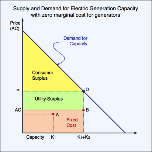
click on image to obtain high-resolution PDF version

Capacity in the first diagram appears insufficient. What happens when the electric utility builds a third power plant? This case is illustrated in the second diagram below. Average cost and capacity move from point B to point C. The average cost goes up a little, indicating that the third power plant is perhaps in a less favourable location than the first two power plants. However, as there is now sufficient capacity available to satisfy demand, retail price and average cost become equal. The green utility surplus vanishes, and consumer surplus increases. The downside is that we must pay the total cost of maintaining capacity at point C, not at point D. This excess capacity is an inefficiency. Whereas in the above diagram we had too little capacity, we now have a bit too much. Which situation is better? First note that in the second diagram there is no producer surplus. Generating capacity is sold "at cost".

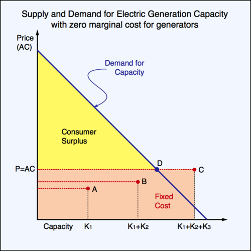
click on image to obtain high-resolution PDF version

Which of the two solutions is better depends on the specific parameters in the model. Moving from two to three generators, consumers gain more surplus, but the producer surplus disappears. Whether there is a net gain is a matter of crunching numbers. In the first diagram, welfare—the sum of consumer surplus and producer surplus—is equal to the yellow triangle and the green rectangle: \[W^{(2)}=\frac{(a-p^{(2)})^2}{2} +(p^{(2)}-c^{(2)})\cdot K^{(2)}\] where \(c^{(2)}=\rho\cdot F^{(2)}/K^{(2)} \) and \( p^{(2)}=a-b\cdot K^{(2)} \). Thus, \[W^{(2)}= a\cdot K^{(2)}+(b^2/2-b)\cdot (K^{(2)})^2 -\rho\cdot F^{(2)} \] In the second diagram, welfare is simply equal to the consumer surplus triangle and therefore \[W^{(3)}=\frac{1}{2}\left( a-\rho\frac{F^{(3)}}{K^{(3)}}\right)^2\] When \(W^{(3)}\) is larger than \(W^{(2)}\), the additional capacity should be installed. The expression \(W^{(3)}-W^{(2)}\) does not simplify further. Determining the outcome of the welfare comparison requires numerical calculations.

What happens when the demand for capacity shifts to the right, for example when the population is growing? Mathematically, this means that parameter \(a\) increases. If we already have three power plants, the extra capacity demand only increases the consumer surplus. The reserve margin allows a higher utilization of the existing capacity. This should actually lower the price of energy, as the cost for capacity is now divided among more consumers.

A key question in the discussion above is how much excess capacity the utility should put into place. How far out should point C be relative to point D in anticipation of population growth? There is a trade-off. If the utility expands capacity just enough to meet current demand, the average cost may not rise much. If the utility puts into place a much larger project, the average cost of capacity may rise more significantly. This is an intertemporal optimization problem. Too much unused capacity today has to be paid for today, but this may be the result of technological constraints. Large hydro dams, for example, cannot be divided into many smaller dams. However, technology may help find alternatives to large-scale projects. Smaller run-of-the-river dams, geothermal power plants, and wind farms, may provide smaller steps to expand capacity, preventing point C to move too far ahead of point D. On the other hand, if a large project can deliver significant economies of scale that smaller projects cannot, the lower average cost will prioritize it over smaller projects. Keep in mind that projects should be entered in sequence of their average cost, regardless of their size.

Situations with zero marginal costs make for interesting economics. They will change the business model that is required to succeed in such markets. In many instances, conventional markets that approach zero marginal costs will morph into alternative, parallel markets where marginal costs will not be zero. Energy markets will increasingly morph into capacity markets. And you can also expect that this process will bring about the demise of some established businesses, but it will also create new and novel type of businesses.