In our basic environmental economics courses we like to teach pollution abatement in simple terms of marginal abatement costs equal to marginal damage. At the margin, these two concepts explain nicely how putting a price on a negative externality—whether it is carbon dioxide or another pollutant—is the most efficient way to mitigate the negative externality. Reality, of course, is always more complex than we can put into a simple model. Whereas our models focus on emission abatement at the intensive margin where firms can move abatement effort up and down continuously, in practice firms face decisions about abatement effort mostly at the extensive margin: whether to invest in a particular device—a venturi scrubber or an electrostatic precipitator or a carbon-capture device. When investment decisions are discrete, the economics gets a bit more complicated.

The intensive margin of abatement

Let us start with a very simple model with an intensive margin and then introduce the extensive margin as a modification. As in my June 17 blog about EITE industries, consider a firm with output \(q\), linear demand \(p=a-bq/2\), and emission intensity \(e\), The firm faces carbon price \(\tau\) on its total emissions \(e\cdot q\), but has the ability to abate at an increasing cost of \(s\cdot(e^\diamond-e)^2/2\) per unit of output, where \(e^\diamond\) is the unabated emission intensity. Note that the \(e^\diamond-e\) is emissions abated, the difference between the original level and the level the firm chooses. The square in the abatement cost function indicates that it gets harder and harder to achieve more emission reduction. Technically, this means that marginal abatement costs are increasing with the amount of abatement. Production costs have a constant marginal cost \(c\). With this set-up profits are: \[ \pi = (a-bq/2)\cdot q-[c+s\cdot(e^\diamond-e)^2/2+\tau\cdot e]\cdot q \] The first-order condition for a profit maximum implies optimal emission level \(e^\ast\) and optimal emission abatement of \[e^\diamond-e^\ast=\tau/s\] and an optimal output level of \[ q^\ast=\frac{a-c-g(\tau)}{b} \quad\mathrm{with}\quad g(\tau)\equiv\tau \left(e^\diamond-\frac{\tau}{2s}\right) \] At \(\tau=se^\diamond\), abatement is complete and emissions are reduced to zero. At that point output is reduced by \(se^\diamond/2b\) units. At the intensive margin an emission tax achieves its desired effect through two channels: a combination of output reduction and deploying abatement technology.

The extensive margin of abatement

Now let us see what happens when the firm only has a choice between continuing without abatement at emission intensity \(e^\diamond\) or deploy a single abatement technology with emission intensity \( 0<e^\square<e^\diamond\) at a fixed cost of \(f\) for purchasing the devide and a marginal cost \(d\) for operating the device. This decision to deploy or not is the extensive margin of pollution abatement. Deploying abatement is not simply the cost of purchasing the device but also the cost of operating it, which often involves energy use. In other words, abatement affects both total and marginal cost of production. Profits are now two possible scenarios: \[ \pi = \left[a-\frac{b\cdot q}{2}-c\right]\cdot q- \left\{\begin{array}{ll} \tau\cdot e^\diamond\cdot q&\mathrm{without\ abatement}\\ \tau\cdot e^\square\cdot q-d\cdot q-f&\mathrm{with\ abatement} \end{array}\right.\] To make a decision, we need to know profits when we determine optimal output. Regardless of choosing abatement or not, optimal output will be \[ q^\ast=\frac{a-c-\tau\cdot e}{b}\] where of course the emission level is \(e\in\{e^\diamond,e^\square\}\). When the firm chooses to abate, its output will be higher because its emission tax will be lower. Profits will be \[\pi^\diamond=\frac{(a-c-\tau\cdot e^\diamond)^2}{2b}\] with no abatement or \[\pi^\square=\frac{(a-c-d-\tau\cdot e^\square)^2}{2b}-f\] with an abatement device purchased and deployed. The firm will decide to invest in the abatement device when \(\pi^\square>\pi^\diamond\), which is the case when the cost of the abatement device is sufficiently cheap: \[2\cdot f\cdot b<(a-c-d-\tau\cdot e^\square)^2-(a-c-\tau\cdot e^\diamond)^2\] After rearranging expressions a bit one can find that \[2\cdot f\cdot b< [\tau\cdot(e^\diamond-e^\square)-d]\cdot [\tau\cdot(e^\diamond+e^\square)+d-2(a-c)]\] The first term in square brackets on the right hand side of the equation is the benefit from deploying abatement: the emission tax times the emission intensity differential, minus the unit cost of operating the abatement device. The second term in square brackets is a bit trickier to interpret. What we know for sure is that it has to be positive for abatement to be deployed at all. So what is hidden in there is another condition \[\tau> \frac{2(a-c)-d}{e^\diamond+e^\square}\] that tells us that the emission tax has to be high enough to even consider deploying the abatement technology. It is a necessary condition. The sufficient condition is the full expression that includes the fixed cost of the abatement device.

A numerical example

The mathematics above may be daunting for the casual reader of this blog. Don't despair. I will re-frame the information in a graphical version with a simple numerical example. I will simulate a carbon tax from $0/tonne to $30/tonne in the model above with parameters \(a=100\), \(b=1\), \(c=20\), \(d=2\), \(f=240\), \(e^\square=0.2\) and \(e^\diamond=0.5\). Output is scaled by 1,000. This means that deploying the abatement device costs $240,000; it will add 10% to the marginal cost of production; and it will reduce emission intensity by 60%.

First consider profits, as this determines whether abatement technology will be adopted. As the carbon tax rises, profits fall along the blue line without abatement. Initially, profits without abatement are higher than with abatement on the red line. At some point the two lines cross, and abatement is deployed. This happens when the savings from deploying the abatement technology are sufficiently large. The firm will always stay on top of either profit line, indicated in green as the optimal path.

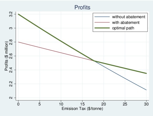
click on image for high-resolution PDF version

Next consider output. Because the firm has no other option at low levels of the carbon tax, it will reduce output to compensate for the increasing tax, which is passed on to consumers in the form of higher prices. Output falls more rapidly without abatement (blue line) than with abatement (red line) because of the different emission intensities. Output moves along the blue line first and then jumps to the red line when the firm finds it worthwhile to deploy abatement. The green line indicates the optimal output path. The moment abatement is deployed, output jumps up as now the firm pays less in carbon taxes.

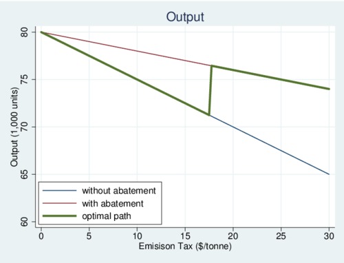
click on image for high-resolution PDF version

Lastly and most importantly: what happens to emissions? As the firm is stuck on its high emission intensity process when the carbon tax is low, emissions only fall (along the blue line) as output is reduced. In other words, the carbon tax does very little in this range. If the firm had started with abatement technology, emissions would be much lower and would fall only gradually as the carbon tax increased (red line). In practice, the optimal path follows the green line and emission fall only a little at first, then fall dramatically when the abatement technology is deployed, and then decrease very little afterwards.

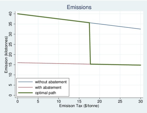
click on image for high-resolution PDF version

It is also useful to ask about the tax efficiency. The measure \[ \Phi\equiv\frac{e^\diamond\cdot q^\diamond -e\cdot q}{\tau\cdot e\cdot q}\] tell us how much emission reduction we are buying for each dollar of tax revenue collected from the firm. The amount \(e^\diamond\cdot q^\diamond \) is the initial emission level without any carbon tax. As emissions fall, the tax efficiency increases. But as the diagram below shows, the tax is rather inefficient at low levels until the abatement technology is deployed. After it is deployed, the efficiency of the tax decreases rapidly as again the only option for the firm is to reduce output in order to reduce emissions further. Obviously, the sweet spot for the carbon tax is the point where the firm deploys abatement technology.

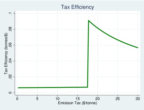
click on image for high-resolution PDF version

Policy implications

The discussions above seem to suggest that a carbon tax is a somewhat problematic instrument as it may depend on hitting the sweet spot where the firms deploy abatement technology. When we aggregate over many firms, this problem diminishes as different firms may all have different emission intensities \(e^\square\) where they deploy abatement technology. When that is the case, the marginal abatement cost curve starts to get smooth again. However, we have a problem when that is not the case and abatement options are "bunched" around a narrow set of technological options. In other words, there is a lack of heterogeneity within an industry. In that case, an emission tax is actually not particularly useful, and it would be much simpler to mandate the best-of-class technology. In that case firms only pay for the abatement technology but are not burdened with extra taxes.

To summarize, many firms make decisions about abatement technology at the extensive margin—whether or not to deploy. At the intensive margin they can only reduce output. An emission tax works well in this situation if different firms within an industry can adopt different technologies. However, an emission intensity standard is preferable when there is only one technological choice for all firms in an industry (e.g., install a state-of-the-art scrubber or not). Emission taxes are best with heterogeneous firms, while emission intensity standards are fine when firms are technologically similar. In the long term, emission taxes have one important advantage, however. They still create an incentive to innovate into abatement technology. After a firm has deployed a current-generation abatement technology, the emission tax that remains will provide a guaranteed return of investment for research and development of the next-generation abatement technology with even lower emission intensity than the current-generation abatement technology.