When you see prices for crude oil moving, how soon do you see these changes reflected in equivalent changes in the price of gasoline at the pump? A common perception is that price increases are passed on quicker than price drops. Is this just a perception or is it real? Do gasoline prices rise like rockets and fall like feathers? Are oil companies colluding to keep prices high, or are there other explanations for asymmetric adjustment speeds?

There is a large string of literature on the rockets-and-feathers hypothesis (RFH). The classic 1991 paper on the topic Rockets and feathers: the asymmetric speed of adjustment of UK retail gasoline prices to cost changes) by Robert Bacon was soon followed by a string of others, notably Borenstein, Cameron, and Gilbertet (1997) that introduced a suitable econometric method for carrying out empirical testing of the RFH. Bachmeier and Griffin (2003) improved some of the econometrics, and their model of asymmetric error correction is what I discuss below. These models have been tweaked in many directions, and I have included a selection of literature below that will provide pointers in these directions.

In general, the evidence on the RFH is mixed. There have been numerous studies that find evidence of rockets and feathers, not only in gasoline markes but also all kinds of other consumer-good markets (Peltzman, 2000). The general wisdom seems to be that markets with high retail-wholesale margins experience a slower adjustment and more asymmetric response (Deltas, 2008). There is also the notion that inventory management can exacerbate the rockets and feathers syndrome. To minimize the capital cost of inventory, gasoline inventory is managed on a "highest in, first out" (HIFO) basis. Inventory with the highest cost of purchase is the first to be used or taken out of stock. As a result, the remaining inventory will have lower cost, and crude oil decreases tend to lower inventory cost before lower prices are passed on to consumers.

When examining the RFH, what matters is also the time horizon. Daily data is more fine-grained than weekly data, and fast adjustment processes may show signs of asymmetry only in daily data but not in weekly data.

But what is the evidence of the RFH in Canada, and in Vancouver specifically? In my April 11 blog I have discussed the pass-through of crude oil prices to the prices you pay at the pump. This pass-through is very effective, but significant deviations from the long-term relationship are possible, and certainly within plus/minus 10 cents.

The asymmetric error-correction model (A-ECM) first estimates a steady-state (long-term) relationship. For gasoline prices \(p_t\equiv\ln(P_t)\) and crude prices \(c_t\equiv\ln(C_t)\), this estimating equation is \[ p_t=\beta_0+\beta_1 c_t +\epsilon_t \] with parameters \(\beta\) and error term \(\epsilon_t\). When reaction speeds ar asymmetric, the cointegrration residuals \(\hat{\epsilon}_t\) and the first differences of the crude price \(\Delta c_t\) can be decomposed into positive and negative values. The second stage of the ECM model is thus estimated as \begin{eqnarray} \Delta p_t& =& \alpha^{+}\hat{\epsilon}^{+}_{t-1} +\alpha^{-}\hat{\epsilon}^{-}_{t-1}\nonumber\\ &&+\sum_{i=0}^m \left(\lambda_i^{+}\Delta c^{+}_{t-i} +\lambda_i^{-}\Delta c^{-}_{t-i}\right)\nonumber\\ &&+\sum_{i=1}^n \left(\theta_i^{+}\Delta p^{+}_{t-i} +\theta_i^{-}\Delta p^{-}_{t-i}\right)+u_t \end{eqnarray} where any variable with a plus superscript is defined as \(z^{+}\equiv\max(0,z)\) and any variable with a minus superscript is defined as \(z^{-}\equiv\min(0,z)\), so that \(z^{+}+z^{-}=z\). The parameters \(\lambda\) and \(\theta\) have corresponding plus and minus subscripts. Furthermore, \(m\) and \(n\) are the number of lags. Formally, the presence of asymmetry can be established by testing the hypotheses that \(\alpha^{+}=\alpha^{-}\), as well as \(\lambda_i^{+}=\lambda_i^{-}\) and \(\theta_i^{+}=\theta_i^{-}\) for all \(i\) using an F-Test.

Below I have taken the data to the test, using 779 weekly observations of West Texas Intermediate crude oil prices (in US$) and Vancouver retail prices of regular gasoline (in cents) between 2000 and 2014. The implementation of the ECM-A model is shown in the SAS code that you find at the bottom of the page, in case you wish to replicate the tests and modify them for your own purposes. The first part of the SAS code generates the required variables using lags and the "min" and "max" operators, followed by the two-step regression with the long-term equilibrium equation and the short-term dynamics equation. The results are then fed into a SAS macro that traces the effect of arbitrary price shocks. The final result is then distilled into the two diagrams shown below.

First, some comments on the two-step regressions. The first equation generates a very good fit, as I had discussed in a previous blog. The \(R^2\) is about 0.90 for the effect of the log price of crude oil on the log retail price of gasoline. The short-term dynamic equation provides a much less impressive fit, only about 0.21. But this is sufficient to estimate the key parameters significantly. A second-order approximation \((m=n=2)\) is entirely sufficient, And additional terms do not show up significantly. Of greatest interest is the F-test that determines whether there is asymmetry in the response to oil prices going up or down. The F-test statistic is reported as 2.67 with an associated P-value of 0.0144. This means that the asymmetry is statistically significant, at roughly the 98% confidence level. But is this difference also economically meaningful?

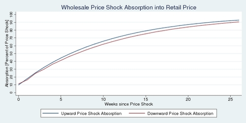
Intepreting each of the estimated coefficients is not straight-forward, and it is much easier to show the effect in a diagram where we simulate +0.1 and –0.1 price shocks. These shocks are in log terms, and represent a 10% increase and 10% decrease in the price of crude oil. The simulation results generate the blue and red curves in the diagram below. They show how the crude oil price shock is absorbed into the retail price over time, 26 weeks in total. To make the vertical axis easier understand, I have expressed it in percentages of full absorption (that is the difference between the original retail price and the new retail price implied by the equlibrium price relationship in the first step of the regression). The diagram shows that it takes about six week for half of the price shock to be absorbed. It's a relatively slow process.

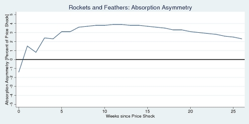
The second diagram highlights the difference between the blue and the red curves. It indicates how much faster the upward movement is relative to the downward movement. The answer to the asymmetry question is: it doesn't matter all that much. At best, the upward movement is about 4% ahead of the downward movement. And in the first week, the downward movement is actually quicker.

Bottom line: the evidence for the rockets-and-feathers hypothesis (RFH) is statistically significant but economically insignificant. It is not enough to get excited about. At least in Vancouver, the RFH is not much to worry about. The rockets are more like the kids version with baking powder and vinegar than the rockets you see in fireworks. Whether other cities show greater asymmetry, that remains for someone else to test. The retail prices of gasoline by city are readily available on the Natural Resources Canada web site.

Data set: CSV file "rockets.csv"; with columns: date (YYYY-MM-DD), crude oil price (US$), and Vancouver retail price for regular gasoline (cents). Right-click and download with the appropriate file name.